In measures of dispersion, the standard deviation is one of the prominent tools to calculate the dispersion of the data
Standard Deviation
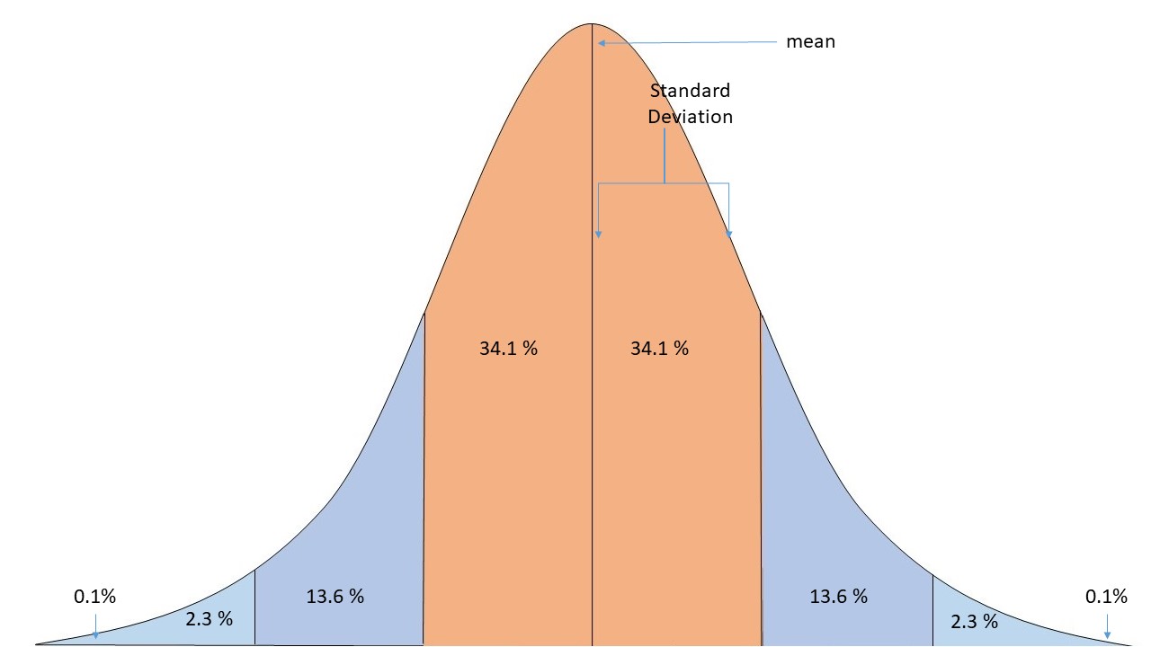
In measures of dispersion, the standard deviation is one of the prominent tools to calculate the dispersion of the data. The purpose of standard deviation is to calculate the deviation of data from the mean of the data. We first calculate the mean of the data, then we sum up the squared difference of each point from the mean.
Simple Data
Let’s directly start with an example of a simple series
34 34 40 43 45 46 48 46
The formula for a standard deviation for Simple Series is as follows, σ is Standard Deviation.
Standard Deviation Formula

In this equation,
N is the number of items in a series, d2 is the Squared differences of items from the series mean
| x | d=| x – μ | | d2 |
|---|---|---|
| 34 | 8.5 | 72.25 |
| 38 | 4.5 | 20.25 |
| 40 | 2.5 | 6.25 |
| 43 | 0.5 | 0.25 |
| 45 | 2.5 | 6.25 |
| 46 | 3.5 | 12.25 |
| 48 | 5.5 | 30.25 |
| 46 | 3.5 | 12.25 |
| Σx=340 , μ = 42.5 | Σd2= 160 |

From the above example, we get an idea of how the standard deviation works in theory and practice. As this is a simple series of data, we directly calculated the difference and deviations.
Although, we also face datasets of multiple types, like continuous and discrete series.
Discrete Data
The series below is a discrete series. This type of data can be explained with x as the value or price and f as the frequency of x’s occurrence.
Let’s say x is the value of an item ordered from a grocery store, and f will be how many units of item x are ordered.
The apples cost $60, and there are 250 apples. So the fx will be, 15000
| χ | ƒ |
| 60 | 250 |
| 62 | 300 |
| 64 | 410 |
| 66 | 500 |
| 67 | 350 |
| 68 | 275 |
| 69 | 150 |
| 70 | 100 |
| 71 | 25 |
| f=2360 |

The calculations in this table for standard derivation are slightly different from the simple series. But the root of the formula is still the same.
| χ | ƒ | ƒχ | d=| χ – μ | | d2 | ƒd2 |
|---|---|---|---|---|---|
| 60 | 250 | 15000 | 5.3 | 28.09 | 7022.5 |
| 62 | 300 | 18600 | 3.3 | 10.89 | 3267 |
| 64 | 410 | 26240 | 1.3 | 1.69 | 692.9 |
| 66 | 500 | 33000 | 0.7 | 0.49 | 245 |
| 67 | 350 | 23450 | 1.7 | 2.89 | 1011.5 |
| 68 | 275 | 18700 | 2.7 | 7.29 | 2004.75 |
| 69 | 150 | 10350 | 3.7 | 13.69 | 2053.5 |
| 70 | 100 | 7000 | 4.7 | 22.09 | 2209 |
| 71 | 25 | 1775 | 5.7 | 32.49 | 812.25 |
| Σƒ=2360 | Σƒχ=154115 | Σƒd2=19318.4 |

Continuous Data
Let’s learn to calculate standard deviation from continuous data. In the following example, we will take a sample of continuous data and apply the standard deviation formula on it.
An example of continuous data can be stocks of a company throughout each month of a year, or the average/cumulative weight of students in a class.
The following example of Classes of IQs and f is the number of students in those classes of IQs
| Class | F |
|---|---|
| 40-50 | 11 |
| 50-60 | 23 |
| 60-70 | 40 |
| 70-80 | 60 |
| 80-90 | 35 |
| 90-100 | 16 |
| 100-110 | 09 |
| 110-120 | 06 |
The formulae for standard deviation are

The First Equation calculates the mean of the series.
The second equation calculates the difference between series and mean.
The third equation calculates standard deviation.
| Class | Frequency f | Mid-value m | fm | d=|m-μ | μ=74.95 | d2 | fd2 |
|---|---|---|---|---|---|---|
| 40-50 | 11 | 45 | 495 | 29.95 | 897 | 9867 |
| 50-60 | 23 | 55 | 1265 | 19.95 | 398 | 9154 |
| 60-70 | 40 | 65 | 2600 | 9.95 | 99 | 3960 |
| 70-80 | 60 | 75 | 4500 | 0.05 | 0.0025 | 0.15 |
| 80-90 | 35 | 85 | 2975 | 10.05 | 101 | 3515 |
| 90-100 | 16 | 95 | 1520 | 20.05 | 402 | 6432 |
| 100-110 | 09 | 105 | 945 | 30.05 | 903 | 8127 |
| 110-120 | 06 | 115 | 690 | 40.05 | 1604 | 9624 |
| Σƒ=200 | Σƒm=14990 | Σƒd2=50699.15 |


From the above calculation we get that average IQ of all students is 74.95, and we get the standard deviation from IQ
If you are still wondering, what will we get from calculating? We can find the spread of the data by comparing the difference between the mean and standard deviation.
Let’s see how the widespread and densely populated data would look.


ANCOVA: Analysis of Covariance with python
ANCOVA is an extension of ANOVA (Analysis of Variance) that combines blocks of regression analysis and ANOVA. Which makes it Analysis of Covariance.
Learn Python The Fun Way
What if we learn topics in a desirable way!! What if we learn to write Python codes from gamers data !!
Meet the most efficient and intelligent AI assistant : NotebookLM
Start using NotebookLM today and embark on a smarter, more efficient learning journey!
Break the ice
This can be a super guide for you to start and excel in your data science career.
Two-Way ANOVA
You only need to understand two or three concepts if you have read the one-way ANOVA article. We use two factors instead of one in a two-way ANOVA.
ANOVA (Analysis of Variance ) part 1
A method to find a statistical relationship between two variables in a dataset where one variable is used to group data.
Basic plots with Seaborn
Seaborn library has matplotlib at its core for data point visualizations. This library gives highly statistical informative graphics functionality to Seaborn.
Matplotlib in python
The Matplotlib library helps you create static and dynamic visualisations. Dynamic visualizations that are animated and interactive. This library makes it easy to plot data and create graphs.
Plotly with Python and R
This library is named Plotly after the company of the same name. Plotly provides visualization libraries for Python, R, MATLAB, Perl, Julia, Arduino, and REST.
Numpy Array
Numpy array have functions for matrices ,linear algebra ,Fourier Transform. Numpy arrays provide 50x more speed than a python list.
NumPy: Python’s Mathematical Backbone
Numpy has created a vast ecosystem spanning numerous fields of science.
Introduction to Pandas: A Guide
Pandas is a easy to use data analysis and manipulation tool. Pandas provides functionality for categorical,ordinal, and time series data . Panda provides fast and powerful calculations for data analysis.
Pandas Dataframe in brief
In this tutorial, you will learn How to Access The Data in Various Ways From the dataframe.
Exploring the World of Sets in Python
Understand one of the important data types in Python. Each item in a set is distinct. Sets can store multiple items of various types of data.
Points You Earned

0 distinction_points

python_points 0
0 Solver points
Leave a Reply
You must be logged in to post a comment.