In measures of dispersion, the standard deviation is one of the prominent tools to calculate the dispersion of the data
Standard Deviation
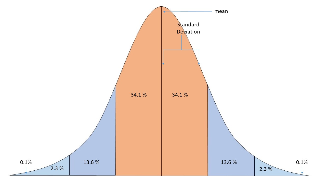
In measures of dispersion, the standard deviation is one of the prominent tools to calculate the dispersion of the data. The purpose of standard deviation is to calculate the deviation of data from the mean of the data. We first calculate the mean of the data, then we sum up the squared difference of each point from the mean.
Simple Data
Let’s directly start with an example of a simple series
34 34 40 43 45 46 48 46
The formula for a standard deviation for Simple Series is as follows, σ is Standard Deviation.
Standard Deviation Formula

In this equation,
N is the number of items in a series, d2 is the Squared differences of items from the series mean
| x | d=| x – μ | | d2 |
|---|---|---|
| 34 | 8.5 | 72.25 |
| 38 | 4.5 | 20.25 |
| 40 | 2.5 | 6.25 |
| 43 | 0.5 | 0.25 |
| 45 | 2.5 | 6.25 |
| 46 | 3.5 | 12.25 |
| 48 | 5.5 | 30.25 |
| 46 | 3.5 | 12.25 |
| Σx=340 , μ = 42.5 | Σd2= 160 |

From the above example, we get an idea of how the standard deviation works in theory and practice. As this is a simple series of data, we directly calculated the difference and deviations.
Although, we also face datasets of multiple types, like continuous and discrete series.
Discrete Data
The series below is a discrete series. This type of data can be explained with x as the value or price and f as the frequency of x’s occurrence.
Let’s say x is the value of an item ordered from a grocery store, and f will be how many units of item x are ordered.
The apples cost $60, and there are 250 apples. So the fx will be, 15000
| χ | ƒ |
| 60 | 250 |
| 62 | 300 |
| 64 | 410 |
| 66 | 500 |
| 67 | 350 |
| 68 | 275 |
| 69 | 150 |
| 70 | 100 |
| 71 | 25 |
| f=2360 |

The calculations in this table for standard derivation are slightly different from the simple series. But the root of the formula is still the same.
| χ | ƒ | ƒχ | d=| χ – μ | | d2 | ƒd2 |
|---|---|---|---|---|---|
| 60 | 250 | 15000 | 5.3 | 28.09 | 7022.5 |
| 62 | 300 | 18600 | 3.3 | 10.89 | 3267 |
| 64 | 410 | 26240 | 1.3 | 1.69 | 692.9 |
| 66 | 500 | 33000 | 0.7 | 0.49 | 245 |
| 67 | 350 | 23450 | 1.7 | 2.89 | 1011.5 |
| 68 | 275 | 18700 | 2.7 | 7.29 | 2004.75 |
| 69 | 150 | 10350 | 3.7 | 13.69 | 2053.5 |
| 70 | 100 | 7000 | 4.7 | 22.09 | 2209 |
| 71 | 25 | 1775 | 5.7 | 32.49 | 812.25 |
| Σƒ=2360 | Σƒχ=154115 | Σƒd2=19318.4 |

Continuous Data
Let’s learn to calculate standard deviation from continuous data. In the following example, we will take a sample of continuous data and apply the standard deviation formula on it.
An example of continuous data can be stocks of a company throughout each month of a year, or the average/cumulative weight of students in a class.
The following example of Classes of IQs and f is the number of students in those classes of IQs
| Class | F |
|---|---|
| 40-50 | 11 |
| 50-60 | 23 |
| 60-70 | 40 |
| 70-80 | 60 |
| 80-90 | 35 |
| 90-100 | 16 |
| 100-110 | 09 |
| 110-120 | 06 |
The formulae for standard deviation are

The First Equation calculates the mean of the series.
The second equation calculates the difference between series and mean.
The third equation calculates standard deviation.
| Class | Frequency f | Mid-value m | fm | d=|m-μ | μ=74.95 | d2 | fd2 |
|---|---|---|---|---|---|---|
| 40-50 | 11 | 45 | 495 | 29.95 | 897 | 9867 |
| 50-60 | 23 | 55 | 1265 | 19.95 | 398 | 9154 |
| 60-70 | 40 | 65 | 2600 | 9.95 | 99 | 3960 |
| 70-80 | 60 | 75 | 4500 | 0.05 | 0.0025 | 0.15 |
| 80-90 | 35 | 85 | 2975 | 10.05 | 101 | 3515 |
| 90-100 | 16 | 95 | 1520 | 20.05 | 402 | 6432 |
| 100-110 | 09 | 105 | 945 | 30.05 | 903 | 8127 |
| 110-120 | 06 | 115 | 690 | 40.05 | 1604 | 9624 |
| Σƒ=200 | Σƒm=14990 | Σƒd2=50699.15 |


From the above calculation we get that average IQ of all students is 74.95, and we get the standard deviation from IQ
If you are still wondering, what will we get from calculating? We can find the spread of the data by comparing the difference between the mean and standard deviation.
Let’s see how the widespread and densely populated data would look.


ANCOVA: Analysis of Covariance with python
ANCOVA is an extension of ANOVA (Analysis of Variance) that combines blocks of regression analysis and ANOVA. Which makes it Analysis of Covariance.
Learn Python The Fun Way
What if we learn topics in a desirable way!! What if we learn to write Python codes from gamers data !!
Meet the most efficient and intelligent AI assistant : NotebookLM
Start using NotebookLM today and embark on a smarter, more efficient learning journey!
Break the ice
This can be a super guide for you to start and excel in your data science career.
A Beginner’s Guide to Immutable Tuples
Tuples are a sequence of Python objects. A tuple is created by separating items with a comma. They are put inside the parenthesis “”(“” , “”)””.
Mastering Python Dictionary: A Beginner’s Guide to Coding Elegance
In this following article we will familiarize with dictionary and it’s numerous functionalities that makes it so versatile.
Decoding Python Byte Sequences: A Beginner’s Guide
Learn to store bytes and byte-arrays. Learn to convert normal datatypes to byte sequence. The bytes() function in Python returns an immutable bytes sequence.
Mastering Print in Python: A Beginner’s Guide to Output, Formatting,
At its heart, the `print()` function sends data to the standard output, typically the console.
Python Lists: A Beginner’s Expedition
List is one of the four data types in Python. Python allows us to create a heterogeneous collection of items inside a list.
Unraveling the Magic of NLP
NLP is a branch of AI that concerns with computers(AI) understanding natural languages.
The Boolean Tapestry: Weaving Logic into Python
Booleans are most important aspects of programming languages.
Everything You Need To Know About Booleans in python
Booleans are most important aspects of programming languages.
Sentiment Analysis
Sentiment analysis can determine the polarity of sentiments from given sentences. We can classify them into certain ranges positive, neutral, negative
Mastering Strings in Python: A Beginner’s Guide
Strings is one of the important fundamental datatypes in python. Interactions of input and output console’s are conveyed using strings.
Points You Earned

0 distinction_points

python_points 0
0 Solver points
Leave a Reply
You must be logged in to post a comment.