Random forest trees combine multiple decision trees to obtain an output. And it is flexible enough to adapt to Classification and Regression.
Random Forest with python
Random forest trees combine multiple decision trees to obtain an output. And it is flexible enough to adapt to Classification and Regression.
Methods that use multiple algorithms for one result are known as ensemble training. Random Forests are one of the ensemble training methods.
As we have touched on the topic of decision trees, let’s have a short discussion on Decision Trees.
Decision Trees
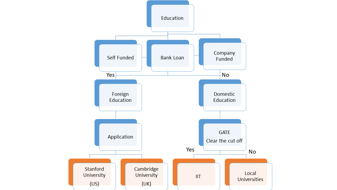
When A decision/situation has two branches like whether to go for foreign education, so branches/threads are yes or no.
If yes which university to approach Stanford: yes/no.
Which bank to approach for a loan, Federal Bank/HDFC Bank? Decision trees help us make multiple decisions in a dataset. Consider a decision tree node as a conditional logic like an if condition.

This way, decisions are made in real life. Similarly, this algorithm mimics the decision-making process by using.
Now let’s consider the same concept with another example.
Example: consider if there’s a space shuttle launch scheduled for tomorrow morning. And the weather forecast tells us there are chances of weather being slightly cloudy but there’s a slight window that makes it so that the shuttle can still be launched within a margin of error.

After you’ve understood the concept of decision trees
Random forest algorithms use multiple trees, but these trees run in parallel. They run independently to generate the same result.
Types of Random Forest Algorithm
- Random Forest Classification
- Random Forest Regressor
Random Forest Classifier
Let’s summarize the decision tree above. We use multiple layers of different factors that play a considerable part in decision-making. Where we start from a root node with the first condition, which reaches out to another two decision nodes and so on. With this as a base, a random forest classifier utilizes multiple decision trees with different subsets of factors. Random Forest Classifier uses multiple decision trees to conclude the same set of decisions. All the multiple decision trees use randomly selected subsets, and the trees get votes on the accuracy of their results. And most popular trees will be chosen to create the final model of the algorithm.
Let’s create and analyse our own implementation of the algorithm.
Python
Python
Python
import pandas as pd
df = pd.read_csv('social_data.csv')| users | age | gender | city | tier | pincode | photos | average likes | average comments | followers | daily user | daily_use_norm | |
|---|---|---|---|---|---|---|---|---|---|---|---|---|
| 0 | 665061268 | 30 | 0 | 18 | 1 | 695676 | 720 | 540 | 22 | 558 | 9861381 | 0 |
| 1 | 670375745 | 17 | 0 | 4 | 2 | 454465 | 237 | 136 | 9 | 144 | 515712 | 1 |
| 2 | 663125396 | 22 | 0 | 19 | 3 | 290159 | 140 | 1254 | 197 | 1311 | 1168320 | 1 |
| 3 | 679258284 | 26 | 0 | 2 | 2 | 347634 | 516 | 104 | 5 | 108 | 1159142 | 1 |
| 4 | 676211941 | 25 | 1 | 10 | 2 | 656937 | 399 | 502 | 32 | 522 | 3267361 | 1 |
| … | … | … | … | … | … | … | … | … | … | … | … | … |
| 1124 | 673315234 | 98 | 0 | 8 | 3 | 535460 | 34 | 47 | 144 | 71 | 787 | 1 |
| 1125 | 663589437 | 42 | 1 | 17 | 2 | 354073 | 35 | 73 | 92 | 107 | 2971 | 1 |
| 1126 | 676728047 | 99 | 1 | 19 | 3 | 411071 | 27 | 18 | 77 | 75 | 473 | 1 |
| 1127 | 661133538 | 63 | 0 | 16 | 2 | 249356 | 34 | 84 | 159 | 116 | 2083 | 1 |
| 1128 | 684290241 | 87 | 1 | 19 | 2 | 381137 | 25 | 39 | 144 | 77 | 521 | 1 |
Python
Python
Python
from sklearn.metrics import accuracy_score,  confusion_matrix, precision_score, recall_score, ConfusionMatrixDisplay
from scipy.stats import randint

X=df.iloc[:,1:-2]
Y=df.iloc[:,-1]
Model creation
In the following code, we are splitting the data into a test train of x and y into 4 different subsets for fitting them in the random forest classification model.
Python
Python
Python
from sklearn.model_selection import RandomizedSearchCV, train_test_split
X_train, X_test, Y_train, Y_test = train_test_split(X, Y, test_size=0.3)
from sklearn.ensemble import RandomForestClassifier
model=RandomForestClassifier()
model.fit(X_train,Y_train)
Output
RandomForestClassifier
RandomForestClassifier()
Model accuracy Evaluation
We will predict the trained model with the test data we extracted before training.
Python
Python
Python
Y_pred = model.predict(X_test)
accuracy = accuracy_score(Y_test, Y_pred)
print("Accuracy:", accuracy)
Output
Accuracy: 0.9705014749262537So we have an accuracy of 97%, yet we do not have any idea how the decision tree structure formed during the training. So the library graphviz will visualize the tree. Following is the code for rendering the decision tree from the trained model.
Python
Python
Python
from sklearn.tree import export_graphviz
from IPython.display import Image
import graphviz
for i in range(1):
    tree = model.estimators_[i]
    dot_data = export_graphviz(tree, feature_names=X_train.columns, filled=True, impurity=False, proportion=True)
    graph = graphviz.Source(dot_data)
    display(graph)
graph.format = 'png'
graph.render('dtree_render',view=True)

Random Forest Regressor
Random forest regression has a similar build as a classifier; it uses multiple decision trees running separately to come to the same result as other trees. In the case of regression, we use the aggregate of all trees to predict an output. These trees use different samples of data and different subsets of columns in a dataset.
In the following example of random forest regression, we will be using the data collected for Moore’s law. Moore’s law says the number of transistors on a microchip will double every year, meanwhile, the cost of a computer will be half of the previous two years. Forget the cost part, we will have the year and number of transistors on a microchip per year since 1971.
Python
Python
Python
import pandas as pd
import numpy as np
import matplotlib.pyplot as pyplot
df=pd.read_csv('moore.csv',names=['year','transistors'])
df
# year and most number of transisitors fit inside a microprocessor.| year | transistors |
|---|---|
| 1971 | 2300 |
| 1972 | 3500 |
| 1973 | 2500 |
| 1973 | 2500 |
| 1974 | 4100 |
| … | … |
| 2017 | 18000000000 |
| 2017 | 19200000000 |
| 2018 | 8876000000 |
| 2018 | 23600000000 |
| 2018 | 9000000000 |
162 rows × 2 columns
Split train and test data
First, we will separate the x and y data. And then split test and train data. We will predict the number of transistors by year.
Python
Python
Python
# seperate
X=df['year']
Y=df['transistors']

# Split train and test data
from sklearn.model_selection import RandomizedSearchCV, train_test_split
X_train, X_test, Y_train, Y_test = train_test_split(X, Y, test_size=0.3)
Model Creation And Training
In following code we will train the random forest regressor. Be mindful that the data will be reshaped to (-1,1)
seperate
X=df[‘year’]
Y=df[‘transistors’]
Split train and test data
Python
Python
Python
# import libraries
from sklearn.ensemble import RandomForestRegressor
regressor = RandomForestRegressor(n_estimators= 10, random_state=0)
# training model
regressor.fit(X.values.reshape(-1,1),Y.values.reshape(-1,1))
RandomForestRegressor(n_estimators=10, random_state=0)
Visualisations
Since this is a regression algorithm, we will visualize this into more traditional regression model representation. With scatter plot of data and line plot predicted from the model.
Python
Python
Python
# create array within range of maximum anad minimum number of
grx = np.arange(min(X), max(X), 0.01)
grx = grx.reshape((len(X_grid), 1))

plt.scatter(X, Y, color = 'cyan')
plt.plot(grx, regressor.predict(grx),color = 'red')
plt.title('Random Forest Regression')
plt.xlabel('Position level')
plt.ylabel('Salary')
plt.show()
ANCOVA: Analysis of Covariance with python
ANCOVA is an extension of ANOVA (Analysis of Variance) that combines blocks of regression analysis and ANOVA. Which makes it Analysis of Covariance.
Learn Python The Fun Way
What if we learn topics in a desirable way!! What if we learn to write Python codes from gamers data !!
Meet the most efficient and intelligent AI assistant : NotebookLM
Start using NotebookLM today and embark on a smarter, more efficient learning journey!
Break the ice
This can be a super guide for you to start and excel in your data science career.
IQR with Excel and python
In this article, we will learn how to utilize the functionalities provided by excel and python libraries to calculate IQR,
Tourism Trend Prediction
After tourism was established as a motivator of local economies (country, state), many governments stepped up to the plate.
Sentiment Analysis Polarity Detection using pos tag
Sentiment analysis can determine the polarity of sentiments from given sentences. We can classify them into certain categories.
For loop with Dictionary
Traverse a dictionary with for loop Accessing keys and values in dictionary. Use Dict.values() and Dict.keys() to generate keys and values as iterable. Nested Dictionaries with for loop Access Nested values of Nested Dictionaries How useful was this post? Click on a star to rate it! Submit Rating
For Loops with python
For loop is one of the most useful methods to reuse a code for repetitive execution.
Metrics and terminologies of digital analytics
These all metrics are revolving around visits and hits which we are getting on websites. Single page visits, Bounce, Cart Additions, Bounce Rate, Exit rate,
Hypothesis Testing
Hypothesis testing is a statistical method for determining whether or not a given hypothesis is true. A hypothesis can be any assumption based on data.
A/B testing
A/B tests are randomly controlled experiments. In A/B testing, you get user response on various versions of the product, and users are split within multiple versions of the product to figure out the “winner” of the version.
For Loop With Tuples
This article covers ‘for’ loops and how they are used with tuples. Even if the tuples are immutable, the accessibility of the tuples is similar to that of the list.
Multivariate ANOVA (MANOVA) with python
MANOVA is an update of ANOVA, where we use a minimum of two dependent variables.
Points You Earned

0 distinction_points

python_points 0
0 Solver points
Leave a Reply
You must be logged in to post a comment.