A method to find a statistical relationship between two variables in a dataset where one variable is used to group data.
ANOVA (Analysis of Variance ) part 1

Definition of ANOVA: A statistical method in which the variation in a set of observations is divided into distinct components. According to Oxford languages.
Simply put, it would be a method to find a statistical relationship between two variables in a dataset where one variable is used to group data.
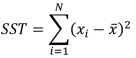
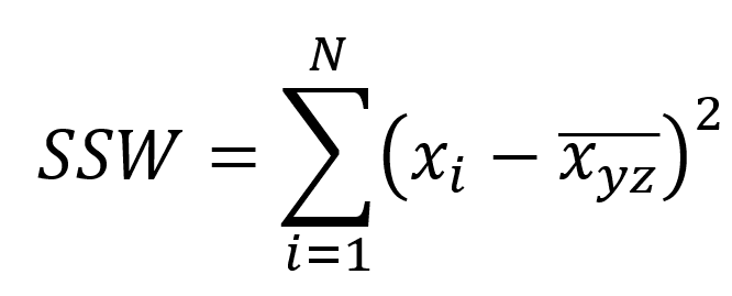
The method to find the statistical significance is to calculate the variance across the whole dataset, the variance between groups, and the variance within groups.
To perform ANOVA on a dataset, we need one categorical and one continuous variable.
Types of ANOVA
- One Way ANOVA
- Two Way ANOVA
One Way ANOVA
One-way ANOVA is used to compare three or more groups based on one categorical and one continuous variable.
Import Required Libraries
import pandas as pd
import numpy as np
import random
# Library to extract f-value
import scipy.stats
Create Dataset
# create random x variable
x=random.sample(range(0, 16), 15)
data={'x':x,'y':[1,1,1,1,1,2,2,2,2,2,3,3,3,3,3]}
df=pd.DataFrame(data)| 0 | 1 | 2 | 3 | 4 | 5 | 6 | 7 | 8 | 9 | 10 | 11 | 12 | 13 | 14 | 15 | 16 | 17 | |
|---|---|---|---|---|---|---|---|---|---|---|---|---|---|---|---|---|---|---|
| x | 2 | 3 | 4 | 3 | 4 | 2 | 20 | 22 | 21 | 20 | 21 | 22 | 35 | 36 | 37 | 36 | 37 | 35 |
| y | 1 | 1 | 1 | 1 | 1 | 1 | 2 | 2 | 2 | 2 | 2 | 2 | 3 | 3 | 3 | 3 | 3 | 3 |
| z | a | a | a | b | b | b | a | a | a | b | b | b | a | a | a | b | b | b |
Let’s start with grouping data. We will group X according to Y.
for i in df['y'].unique():
    print(f'Group {i}')
    print(df[df['y']==i],end='\n\n')
Group 1
   x  y  z
0  2  1  a
1  3  1  a
2  4  1  a
3  3  1  b
4  4  1  b
5  2  1  b

Group 2
     x  y  z
6   20  2  a
7   22  2  a
8   21  2  a
9   20  2  b
10  21  2  b
11  22  2  b

Group 3
     x  y  z
12  35  3  a
13  36  3  a
14  37  3  a
15  36  3  b
16  37  3  b
17 35 3 bCalculating the means of each group
groupM=df.groupby('y').mean().reset_index()
groupM y x
0 1 3.0
1 2 21.0
2 3 36.0Calculate the mean of all data (grand mean)
grandM=df['x'].sum()/15
grandM20.0Calculate the Sum of Squares Total

df['sst']=(df['x']-(df.x.sum()/len(df)))**2
SST=df['sst'].sum()
print(SST)3288.0Calculate the Sum of Squares Within

SSW=0
for i in list(df['y'].unique()):
    #print(i)
    g=pd.DataFrame(df[df['y']==i].x-float(groupM[groupM['y']==i].x))**2
    SSW+=g.sum()
print(float(SSW))
8490.0Calculate Sum of Squares Between
groupM['ssb']=groupM.x-grandM
groupM['ssb']=groupM['ssb']**2
groupM['ssb']=groupM['ssb']*N
SSB=groupM.ssb.sum()
print(SSB)
2730.0All the knowledge that has been obtained up to this point is used to comprehend the occasion, setting, and context as well as the meaning of the statement.
Calculate the Degree of freedom for SST, SSW, SSB
The concept of degree of freedom is a method for comprehending logically independent values. By calculating the degree of freedom, we can get the scope of an interpretable sample of factors in the dataset.
N=len((df[df['y']==1]))
M=len(df['y'].unique())
print(M,N)
3 6 # Degrees of Freedom for all
sstdf= (M*N)-1
sswdf= M*(N-1)
ssbdf= M-1
print(f'DF\n SST= {sstdf}\n SSW= {sswdf}\n SSB= {ssbdf}')
DF
 SST= 17
 SSW= 15
SSB= 2Values Table
Let’s create a table with all the values we have found so far.
final_table=pd.DataFrame({
    'Sum of Squares':[float(SSW),float(SSB),float(SST),np.nan],
    'Degree of Freedom':[sswdf,ssbdf,sstdf,np.nan],
    'Mean Square':[np.nan for x in range(4)],
    'F score':[np.nan for x in range(4)],
    'F Value':[np.nan for x in range(4)],
    'H0':[np.nan for x in range(4)]} ,
    index=['Sum of Squares Within','Sum of Squares Between','Sum of Squares Total','Result'])
final_table| Sum of Squares | Degree of Freedom | Mean Square | F score | F Value | H0 | |
|---|---|---|---|---|---|---|
| Sum of Squares Within | 220.8 | 12.0 | ||||
| Sum of Squares Between | 59.2 | 2.0 | ||||
| Sum of Squares Total | 280.0 | 14.0 | ||||
| Result |
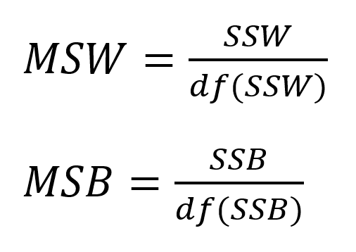
Mean Square
To calculate the mean square, we divide the degree of freedom by the respective sum of squares.

final_table.loc[:'Sum of Squares Between']['Mean Square']=final_table.loc[:'Sum of Squares Between']['Sum of Squares']/final_table.loc[:'Sum of Squares Between']['Degree of Freedom']
final_table| Sum of Squares | Degree of Freedom | Mean Square | F score | F Value | H0 | |
|---|---|---|---|---|---|---|
| Sum of Squares Within | 220.8 | 12.0 | 18.4 | |||
| Sum of Squares Between | 59.2 | 2.0 | 29.6 | |||
| Sum of Squares Total | 280.0 | 14.0 | ||||
| Result |
F score and F value
We can calculate the f score by dividing the mean square of between by the mean square of within. The square value will be in the scope of f distribution. After finding f value via the degree of freedom. We can determine whether the null hypothesis is rejected or accepted.


# F score
final_table['F score']['Result']=final_table['Mean Square']['Sum of Squares Between']/final_table['Mean Square']['Sum of Squares Within']

# F value
numerator=final_table['Degree of Freedom']['Sum of Squares Between']
denominator=final_table['Degree of Freedom']['Sum of Squares Within']
alpha=0.05
final_table['F Value']['Result']=scipy.stats.f.isf(alpha, numerator, denominator)

# Reject or fail to Reject Null hypothesis
final_table['H0']['Result']=final_table['F score']['Result']<final_table['F Value']['Result']
final_table| Sum of Squares | Degree of Freedom | Mean Square | F score | F Value | H0 | |
|---|---|---|---|---|---|---|
| Sum of Squares Within | 220.8 | 12.0 | 18.4 | |||
| Sum of Squares Between | 59.2 | 2.0 | 29.6 | |||
| Sum of Squares Total | 280.0 | 14.0 | ||||
| Result | 1.608696 | 3.885294 | True |
So the null hypothesis is accepted in this instance. Try to run this program on your system. Your result may vary because our X is produced randomly.
Make a note that terms regarding null hypotheses are “reject the null hypothesis” or “fail to reject the null hypothesis.” But for ease of understanding, we used rejection or acceptance.
Learn Python The Fun Way
What if we learn topics in a desirable way!! What if we learn to write Python codes from gamers data !!
Meet the most efficient and intelligent AI assistant : NotebookLM
Start using NotebookLM today and embark on a smarter, more efficient learning journey!
ANCOVA: Analysis of Covariance with python
ANCOVA is an extension of ANOVA (Analysis of Variance) that combines blocks of regression analysis and ANOVA. Which makes it Analysis of Covariance.
Break the ice
This can be a super guide for you to start and excel in your data science career.
Diffusion Models: Making AI Creativity
Stable Diffusion Models: Where Art and AI Collide Artificial Intelligence meets creativity in the fascinating realm of Stable Diffusion Models. These innovative models take text descriptions and bring them to life in the form of detailed and realistic images. Let’s embark on a journey to understand the magic behind Stable Diffusion in a way that’s…
Quiz Challenge: Basics with Python [Questions]
Solve These Questions in Following Challange
Introducing Plethora of Stable Diffusion models: Part 1
Generate AI images as good as DALL-E completely offline.
Understanding Demand Forecasting and Addressing Common Challenges
Are demand forecasting truly predictable? Or are they changing randomly?
The Realistic though Dramatic story of AI Superstar
Let’s enjoy the highly interesting story of Tech Superstar chronologically.
Start Your Python Journey from Scratch
starting your Python journey from scratch is a fantastic endeavour.
5 ways to Improve yourself as a Technical Professional
Try learning a topic from basic > if not understood, ask somebody>
10 Ways To Stay Excellent When Exams Are Near
A friendly guide what every computer science student should have when exams are coming
One response to “ANOVA (Analysis of Variance ) part 1”
[…] only need to understand two or three concepts if you have read the ANOVA Part-1 article. We use two factors instead of one in a two-way ANOVA. What this means is that there will […]
Points You Earned


Leave a Reply
You must be logged in to post a comment.