You only need to understand two or three concepts if you have read the one-way ANOVA article. We use two factors instead of one in a two-way ANOVA.
Two-Way ANOVA

You only need to understand two or three concepts if you have read the ANOVA Part-1 article. We use two columns instead of one in a two-way ANOVA. This basically means there will be two categorical columns and one continuous column. We will examine the differences between the two categories, both individually and collectively. As a result, we have three null hypotheses to accept or reject. Furthermore, for each null hypothesis, there is an alternate hypothesis.
With each term we derive, we will highlight a solved example using programming and mathematical denotations.
| x | 20 | 15 | 21 | 14 | 5 | 9 | 16 | 13 | 6 | 11 | 10 | 17 | 18 | 7 | 19 | 8 | 22 | 12 |
|---|---|---|---|---|---|---|---|---|---|---|---|---|---|---|---|---|---|---|
| y | 1 | 1 | 1 | 1 | 1 | 1 | 2 | 2 | 2 | 2 | 2 | 2 | 3 | 3 | 3 | 3 | 3 | 3 |
| z | a | a | a | b | b | b | a | a | a | b | b | b | a | a | a | b | b | b |
This is the dataset we’ll use to demonstrate two-way ANOVA.
This dataset has
- The x column in this dataset represents our continuous factor.
- The categories 1, 2, and 3 are divided equally in y column.
- The categories a and b in the z column are divided equally.
In total, we have 18 rows and 3 columns
Hypothesis: 1
H0 : y has no effect on x.
Ha : y has effect on x.
Hypothesis: 2
H0 : z has no effect on x.
Ha : z has effect on x.
Hypothesis: 3
H0 : y and z combined has no effect on x.
Ha : y and z combined has effect on x.
Data Preparation
Let’s begin by entering the data into a program
# To handle mathematical operations
import numpy as np
# To handle data operations
import pandas as pd
# To find F value.
import scipy.stats

# Data
x=random.sample(range(0, 13), 12)
anov={'x':x,
      'y':[1,1,1,1,1,1,2,2,2,2,2,2,3,3,3,3,3,3],
      'z':['a','a','a','b','b','b','a','a','a','b','b','b','a','a','a','b','b','b']
      }
df=pd.DataFrame(anov)
print(df) x y z
0 14 1 a
1 6 1 a
2 10 1 b
3 9 1 b
4 15 2 a
5 8 2 a
6 7 2 b
7 11 2 b
8 16 3 a
9 13 3 a
10 12 3 b
11 5 3 bMean Table
Compute the means for each category combination
av_tab=df.groupby(['y','z'])['x'].mean().reset_index()
print(av_tab) y z x
0 1 a 18.666667
1 1 b 9.333333
2 2 a 11.666667
3 2 b 12.666667
4 3 a 14.666667
5 3 b 14.000000Individual Means
Compute the means for each category combination
Y Mean
We should use the basic mean formula to get the mean for each category of y. In Python, we will use group-by to achieve the same result.

y_mean=av_tab.groupby('y')['x'].mean().reset_index()
y_mean y x
0 1 14.000000
1 2 12.166667
2 3 14.333333Z Mean
This will be a procedure similar to Y Mean.

z_mean=av_tab.groupby('z')['x'].mean().reset_index()
z_mean z x
0 a 15.0
1 b 12.0Sum Of Squares
The sum of squares is an important part of statistical analysis. The sum of squares is used to compare relationships between factors.
The sum of squares principle states that the group mean should be subtracted from the observations. And squaring it.
By doing so, we will get the variance of the observations from the mean. We can deduce relationships between data by analysing such a sum of squares.
Sum Of Squares of First Factor
To find the sum of the squares of the first factor, use We cumulate a squared series, which is created by subtracting the grand mean from all group means. This subtraction is repeated to match the number of observations with the first factor.
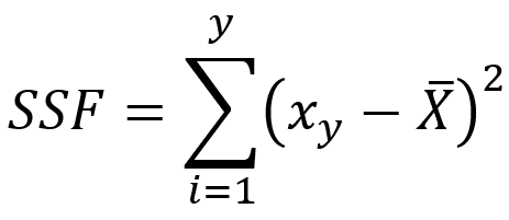
df['ssf']=df['y']
mean_vals=dict([(i, float(y_mean[y_mean['y']==i]['x']) ) for i in df['y'].unique()])
df = df.replace({"ssf": mean_vals})
SSF=(df['ssf']-(df['x'].sum()/len(df)))**2
SSF=SSF.sum()
print(SSF)16.333333333333332Sum of Squares of Second Factor
The sum of squares for the second factor. This operation will be similar to the first factor; the only difference will be that we will use the second factor this time.
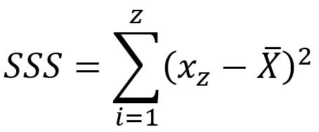
df['SSS']=df['z']
mean_vals=dict([(i, float(z_mean[z_mean['z']==i]['x']) ) for i in df['z'].unique()])
df = df.replace({"SSS": mean_vals})
SSS=(df['SSS']-(df['x'].sum()/len(df)))**2
SSS=SSS.sum()
print(SSS)40.5Sum of squares within
The sum of squares within the groups. We subtract the sub means of y and z combined and subtract the length of their respective yz combos. And square each iteration to get one answer.
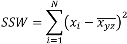
df['yz']=df['y'].astype('str')+df['z']
submean=0
for i in df['yz'].unique():
    submean=df[df['yz']==i]['x'].sum()/len(df[df['yz']==i])
    df=df.replace({'yz':{i:submean}})
SSW=(df['x']-df['yz'])**2
SSW=SSW.sum()
print(SSW)335.33333333333337Sum of Squares Total
To calculate the total sum of squares, we subtract the grand mean from each observation, square the difference, and cumulate over the data.
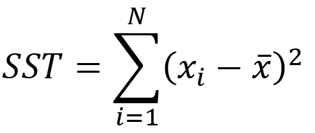
SST=((df['x']-df['x'].sum()/len(df))**2).sum()
print(SST)484.5Sum of Squares of Both Factors
Sum of squares of both factors can be calculated a by a different formula too. But we will use the following formula for ease of understanding and reduction of calculations.

SSB=SST-SSF-SSS-SSW
print(SSB)
92.33333333333331Degree of Freedom
Degree of Freedom for Y
Ny denotes the number of observations in y columns across various categories.

ssfdf=len(df['y'].unique())-1
print(ssfdf)2Degree of Freedom for Z
Nz means the number of observations for z column categories.

sssdf=len(df['z'].unique())-1
print(sssdf) 1Degree of Freedom within
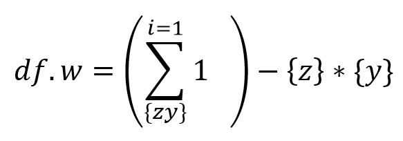
To calculate the degree of freedom for the sum of squares within, we will count the number of unique combination repeats in the data. And subtract that from the product of each category set length.
{y} is the length of the y category set.
{z} is the length of the z category set.
{zy} unique combinations of each category
df['ssf']=df['y'].astype('str')+df['z']
sswdf=df['ssf'].value_counts().sum() - (len(df['y'].unique())*len(df['z'].unique()))
print(sswdf)
12Sum Of Square Degree of Freedom Both Factors
to get d.f.B we multiply df. y and df. z

ssbdf=ssfdf*sssdf
print(ssbdf)2Degree of Freedom for a total sum of square
you use d.f.T to find errors and mistakes in prior calculations.

sstdf= sssdf + ssfdf + sswdf + ssbdf
print(sstdf)17Values Table
We can now concentrate on calculating multiple values at once. Based on current values, we will calculate more. Let’s create a table to record these values to facilitate calculation.
final_table=pd.DataFrame({
    'Sum of Squares':[SSF,SSS,SSB,SSW,SST],
    'Degree of Freedom':[ssfdf,sssdf,ssbdf,sswdf,sstdf],
    'Mean Square':[np.nan for x in range(5)],
    'F score':[np.nan for x in range(5)],
    'F Value':[np.nan for x in range(5)],
    'H0':[np.nan for x in range(5)]} ,
    index=['Sum of Squares Y','Sum of Squares Z','Sum of Squares Both','Sum of Squares Within','Sum of Squares Total'])
print(final_table)| Sum of Squares | Degree of Freedom | Mean Square | F score | F Value | H0 | |
|---|---|---|---|---|---|---|
| Sum of Squares Y | 16.333333 | 2 | ||||
| Sum of Squares Z | 40.500000 | 1 | ||||
| Sum of Squares Both | 92.333333 | 2 | ||||
| Sum of Squares Within | 335.333333 | 12 | ||||
| Sum of Squares Total | 484.500000 | 17 |
Mean Square
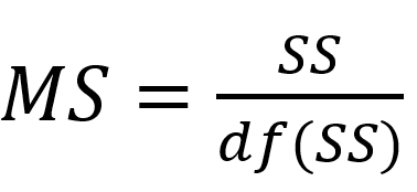
Calculate the Mean Square of the sum of squares. To achieve the mean square, we need to divide the sum of squares by their respective degrees of freedom.
final_table['Mean Square']=final_table.loc[:'Sum of Squares Within']['Sum of Squares']/final_table['Degree of Freedom']
final_table| Sum of Squares | Degree of Freedom | Mean Square | F score | F Value | H0 | |
|---|---|---|---|---|---|---|
| Sum of Squares Y | 16.333333 | 2 | 8.166667 | |||
| Sum of Squares Z | 40.500000 | 1 | 40.500000 | |||
| Sum of Squares Both | 92.333333 | 2 | 46.166667 | |||
| Sum of Squares Within | 335.333333 | 12 | 27.944444 | |||
| Sum of Squares Total | 484.500000 | 17 |
F Score
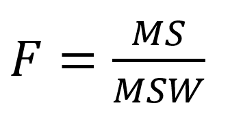
Determine the F score. Now we will find the F score for x, y, and both factors interactions. By dividing the mean square of sum of squares within from all other mean squares.
final_table['F score']=final_table.loc[:'Sum of Squares Both']['Mean Square']/final_table.loc['Sum of Squares Within']['Mean Square']| Sum of Squares | Degree of Freedom | Mean Square | F score | F Value | H0 | |
|---|---|---|---|---|---|---|
| Sum of Squares Y | 16.333333 | 2 | 8.166667 | 0.292247 | ||
| Sum of Squares Z | 40.500000 | 1 | 40.500000 | 1.449304 | ||
| Sum of Squares Both | 92.333333 | 2 | 46.166667 | 1.652087 | ||
| Sum of Squares Within | 335.333333 | 12 | 27.944444 | |||
| Sum of Squares Total | 484.500000 | 17 |
F value and Hypothesis Testing
Let’s find the f value, compare the f-score, and reject/suggest the Hypothesis. There are ways to manually find the f value from an f distribution table. But you will need to automate this process, so use the following method.
for i in final_table.index[:3]:
    print(final_table['Degree of Freedom'][i])
    numerator=final_table['Degree of Freedom'][i]
    denominator=final_table.loc['Sum of Squares Within']['Degree of Freedom']
    final_table['F Value'][i]=scipy.stats.f.isf(0.05, numerator,denominator)
    if final_table['F score'][i] < final_table['F Value'][i]:
        final_table['H0'][i]=True
    else:
        final_table['H0'][i]=False
print(final_table)| Sum of Squares | Degree of Freedom | Mean Square | F score | F Value | H0 | |
|---|---|---|---|---|---|---|
| Sum of Squares Y | 16.333333 | 2 | 8.166667 | 0.292247 | 3.885294 | True |
| Sum of Squares Z | 40.500000 | 1 | 40.500000 | 1.449304 | 4.747225 | True |
| Sum of Squares Both | 92.333333 | 2 | 46.166667 | 1.652087 | 3.885294 | True |
| Sum of Squares Within | 335.333333 | 12 | 27.944444 | |||
| Sum of Squares Total | 484.500000 | 17 |
Because this is randomly generated data, there is a low chance that there is any relation between x, y, and z. So the conclusion seems accurate.
Z has no effect on x.
Y has no effect on X.
You can use the code above to perform a two-way ANOVA on any set of data. Given that you changed the names of categorical columns to y and z and continuous data to x,
ANCOVA: Analysis of Covariance with python
ANCOVA is an extension of ANOVA (Analysis of Variance) that combines blocks of regression analysis and ANOVA. Which makes it Analysis of Covariance.
Learn Python The Fun Way
What if we learn topics in a desirable way!! What if we learn to write Python codes from gamers data !!
Meet the most efficient and intelligent AI assistant : NotebookLM
Start using NotebookLM today and embark on a smarter, more efficient learning journey!
Break the ice
This can be a super guide for you to start and excel in your data science career.
Model Context Protocol (MCP) — the “USB” for AI tools
MCP is the USB port for AI — A standard that lets models like ChatGPT safely connect to tools and servic
Manova Quiz
Solve this quiz for testing Manova Basics
Quiz on Group By
Test your knowledge on pandas groupby with this quiz
Visualization Quiz
Observe the dataset and try to solve the Visualization quiz on it
Versions of ANCOVA (Analysis Of Covariance) with python
To perform ANCOVA (Analysis of Covariance) with a dataset that includes multiple types of variables, you’ll need to ensure your dependent variable is continuous, and you can include categorical variables as factors. Below is an example using the statsmodels library in Python: Mock Dataset Let’s create a dataset with a mix of variable types: Performing…
Python Variables
How useful was this post? Click on a star to rate it! Submit Rating
A/B Testing Quiz
Complete the code by dragging and dropping the correct functions
Python Functions
Python functions are a vital concept in programming which enables you to group and define a collection of instructions. This makes your code more organized, modular, and easier to understand and maintain. Defining a Function: In Python, you can define a function via the def keyword, followed by the function name, any parameters wrapped in parentheses,…
Python Indexing: A Guide for Data Science Beginners
Mastering indexing will significantly boost your data manipulation and analysis skills, a crucial step in your data science journey.
Points You Earned


Leave a Reply
You must be logged in to post a comment.