MANOVA is an update of ANOVA, where we use a minimum of two dependent variables.
Multivariate ANOVA (MANOVA) with python

Think of MANOVA as a more advanced version of ANOVA. While ANOVA looks at one outcome, MANOVA looks at several outcomes at once. It’s like comparing the performance of students in multiple subjects instead of just one.
When we import a dataset, the dataset will have multiple dependent variables and one independent variable. So in MANOVA, we find out if an independent variable affects multiple independent variables. A one-way ANOVA had one dependent and one independent variable, whereas a two-way ANOVA had one dependent and multiple independent variables.
Wilk’s lambda: Wilk’s lambda is a test with some similarities to the f-test. That aids in the final determination of the hypothesis. We will have values similar to the f-test like the alpha value, denominator, numerator, significance value, and F-value. In this test, we will utilise the matrices.
e.g. Wilk’s Lambda is like a referee in a sports game. It checks if the differences in performance (variance) within teams (groups) are significant compared to the differences between teams.
In the Wilks test, we create functions for each group, where the functions are constrained to separate groups. Then we calculate the distinctiveness of the groups as measured by functions.
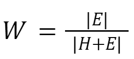
The following function will be used to calculate the Wilks value: E is the sum of squares and cross-product terms for within, and H is the sum of squares. Sum of Squares and Cross Product (SSCP) terms for between. Both of them are triangular matrices.
The final result of Wilks’ test is best when the value is as close to 0 as possible. The PR>F value determines the significance of the test.
0.000 means 100% significance,
and 1.0 means 0% significance.

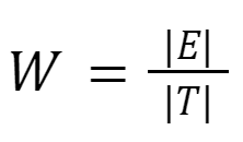
In the following equation, |E| denotes the determinant within SSCP. |E| This gives us the matrix of variance within groups. It is also called an error in samples. In the following equation, H denotes the determinant between SSCP. |H| This gives us the matrix of variance between groups. When we add, |H|+|E| it provides the value of the total sum of squares cross product |T|.
The above equation could also be shown as.

Since MANOVA is a little more complicated than other methods, we will take the iris dataset from the sklearn library here for example since it is familiar.
Sepal length, Sepal width, Petal length and Petal width, are dependent columns with fractal values
A species variable is an independent variable which points to species.
So the first step is what we did in ANOVA. Let’s formulate a hypothesis.
Null Hypothesis (H0): sepal length, sepal width, petal length, and petal width do not have any effect on species.
Alternative Hypothesis (HA): sepal length, sepal width, petal length, and petal width do have a distinguishable effect on species.
import pandas as pd
import numpy as np
import sklearn.datasets as datasets

dataset=load_iris()
df=pd.DataFrame(data=dataset.data,columns=dataset.feature_names)
df['species']=dataset['target']
df=df.rename(columns={'sepal length (cm)':'sl','sepal width (cm)':'sw','petal length (cm)':'pl','petal width (cm)':'pw'})
df.head(5)| sl | sw | pl | pw | species | |
|---|---|---|---|---|---|
| 0 | 5.1 | 3.5 | 1.4 | 0.2 | setosa |
| 1 | 4.9 | 3.0 | 1.4 | 0.2 | setosa |
| 2 | 4.7 | 3.2 | 1.3 | 0.2 | setosa |
| 3 | 4.6 | 3.1 | 1.5 | 0.2 | setosa |
| 4 | 5.0 | 3.6 | 1.4 | 0.2 | setosa |
We will be using the stats model library in the following example
!pip install statsmodelLet’s apply MANOVA to the species dataset. We need to provide dependent and independent variables as a string equation in the “MANOVA.from_formula” function.
Equation building works as follows:
‘Independent_var1 + independent_var2 ~ dependent_var’
‘sl + sw + pl + pw ~ species’
Use the column values from the dataset in the equation.
If you have multiple independent variables. The equation Should look like this
‘group1 + group2 ~ x1 + x2 + x3 + x4’
from statsmodels.multivariate.manova import MANOVA
fit = MANOVA.from_formula('sl + sw + pl + pw ~ species', data=df)
print(fit.mv_test())
                  Multivariate linear model
================================================================

----------------------------------------------------------------
       Intercept         Value  Num DF  Den DF   F Value  Pr > F
----------------------------------------------------------------
          Wilks' lambda  0.0170 4.0000 144.0000 2086.7720 0.0000
         Pillai's trace  0.9830 4.0000 144.0000 2086.7720 0.0000
 Hotelling-Lawley trace 57.9659 4.0000 144.0000 2086.7720 0.0000
    Roy's greatest root 57.9659 4.0000 144.0000 2086.7720 0.0000
----------------------------------------------------------------

----------------------------------------------------------------
        species          Value  Num DF  Den DF   F Value  Pr > F
----------------------------------------------------------------
          Wilks' lambda  0.0234 8.0000 288.0000  199.1453 0.0000
         Pillai's trace  1.1919 8.0000 290.0000   53.4665 0.0000
 Hotelling-Lawley trace 32.4773 8.0000 203.4024  582.1970 0.0000
    Roy's greatest root 32.1919 4.0000 145.0000 1166.9574 0.0000
================================================================In the above output, if you read the second table, Wilk’s first value is 0.0234, which is very close to zero. Which proves there is a significant variance between groups. However, this test does not reveal which groups are distinct from others.
Post-Hoc analysis
LDA (linear discriminant analysis):
The value of 0.0234 is close to 0. So we understand that there is a very significant distinction between groups. But we don’t know which dependent variable combinations separate species. Imagine LDA as a sorting hat from Harry Potter. It helps to place students (data points) into the right houses (groups) based on their characteristics (dependent variables).
from sklearn.discriminant_analysis import LinearDiscriminantAnalysis as lda
x = df[["sl", "sw","pl","pw"]]
y = df["species"]
post_hoc = lda().fit(X=X, y=y)priors_: Priors contain class proportions that are referred from data.
post_hoc.priors_
array([0.33333333, 0.33333333, 0.33333333])
means_: Means of each groups with each variable
post_hoc.means_
array([[5.006, 3.428, 1.462, 0.246],
       [5.936, 2.77 , 4.26 , 1.326],
       [6.588, 2.974, 5.552, 2.026]])
scalings_: These are used to form linear discriminant decision rules.
post_hoc.scalings_
array([[ 0.82937764,  0.02410215],
       [ 1.53447307,  2.16452123],
       [-2.20121166, -0.93192121],
       [-2.81046031,  2.83918785]])
explained_variance_ratio_: Variance ratio calculated between each component.
post_hoc.explained_variance_ratio_
array([0.9912126, 0.0087874])LDA Plot
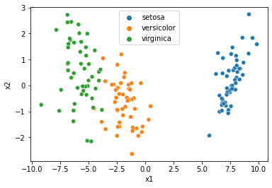
Let’s plot the LDA data. This plot will help us see which groups are more separate than others. To make things clearer, we use the Iris dataset, which is like a garden with different types of flowers. MANOVA and LDA help us understand how these flowers differ based on their features like petal length and width.
import matplotlib.pyplot as plt
import seaborn as sns
lda = pd.DataFrame(lda().fit(X=x, y=y).transform(X), columns=["X1", "X2"])
lda["species"] = df["species"]
sns.scatterplot(data=lda, x="X1", y="X2", hue=df.species.tolist())
plt.show()
In the above plot, you will see that Setosa is distinctive from Versicolor and Virginia.
Serosa stands apart from these two, and we have enough evidence to reject the null hypothesis.
Manova Quiz
Solve this quiz for testing Manova Basics
Multivariate ANOVA (MANOVA) with python
MANOVA is an update of ANOVA, where we use a minimum of two dependent variables.